Application Notes, January 2024
Numerical Modeling of Physical Vapor Deposition:
Capture All That Matter
Physical vapor deposition (PVD), as a manufacturing method, is being employed in a growing list of industries for such products as OLED displays and high-capacity batteries. A preferred approach to PVD engineering is a workflow that incorporates numerical modeling with good realism.
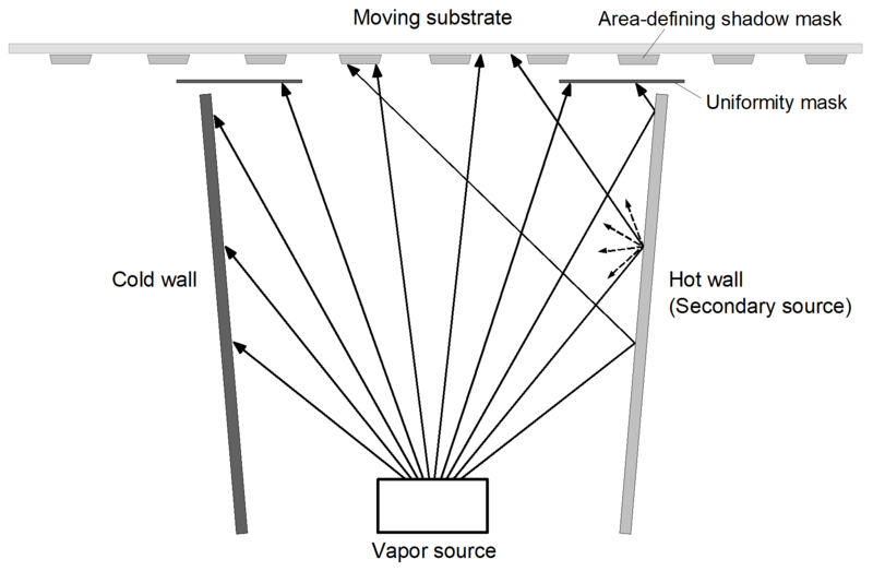
In real-world processes, a number of physical elements can affect the deposition of material layers. The above diagram illustrates what a "real-world" process may entail.
The vapor source may be a large-area crucible, a sputtering target or a point-like source (i.e. an effusion cell); there usually are walls or partitions to confine the material vapor in a space – these wall can be cold or hot; correction masks may be present for achieving uniform thickness; substrates may move in one fashion or another (rotation or translation); and there may be area-defining shadow masks that are affixed to the substrates.
To accurately predict the outcome of a deposition process all the above-mentioned elements must be included in a numerical model. To build such a model from scratch is extremely tedious and time-consuming. A numerical model that allows for rapid assessment of engineering choices is even harder to construct. In the following we turn to a V-Grade 5S series program (Tin Model LLC) for simulating the process shown in Fig.1. We will pay special attention to the difference between cold walls and hot walls.
A cold wall condenses the material vapor it intercepts, much like a substrate. A hot wall, in contrast, re-evaporates all the vapor particles that impinge on it. A cold wall can be modeled as a vapor-obstruction mask (V-Grade 5S series programs can handle vapor-obstruction masks located anywhere). A hot wall, on the other hand, should be treated as a secondary vapor source.
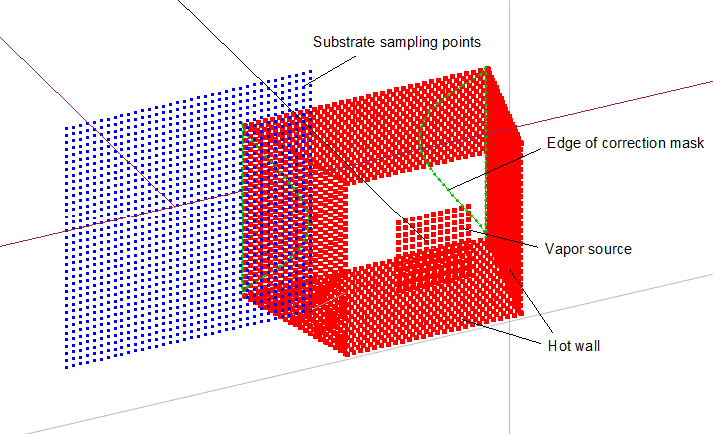
Figure 1
A hot wall can be modeled in V-Grade 5S through these steps:
1) Place a substrate that covers the surface of the hot wall;
2) Compute the thickness distribution formed on the substrate with the primary vapor source;
3) Create a new source surface that overlaps with the hot wall;
4) Assign emittance values to the hot wall with data obtained in Step 2; and
5) Include the hot wall (a secondary source) in the overall source configuration.
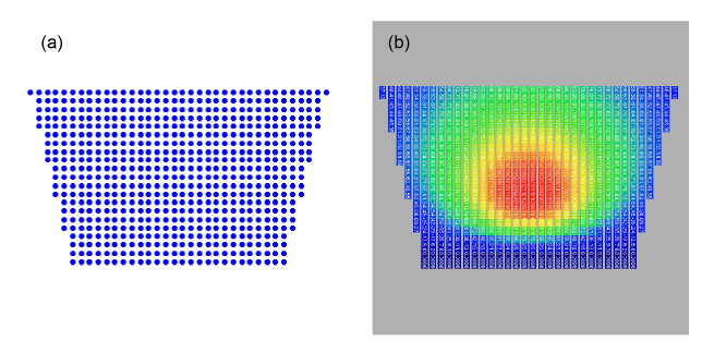
In the example shown in Fig. 2, a screenshot of the 3D chamber view of V-Grade 5S, the primary source is a rectangular-pan evaporator. Surrounding the source are four walls, which are heated to avoid vapor condensation. Because these walls reemit vapor particles originated from the primary source they should be considered secondary vapor sources. To construct the back-wall secondary source, for example, we first introduce a substrate in place of the trapezoid wall as shown in Fig. 3(a); the software program is run to obtain the condensation map shown in Fig. 3(b); values are then extracted from the map to be converted to the emittance values of the back wall. (The V-Grade 5S program allows us to determine that for each gram of material vaporized from the primary source 0.18 gram is intercepted by the back wall and reemitted into the space.)
Figure 2
We repeat the steps for all four walls to complete the source configuration, which includes the primary and the four secondary source planes, as represented by the red points in Fig 2. (Emittance strengths are not visualized in this view). To a substrate, the vapor particles reemitted by the hot walls, or the secondary sources, arrive at large angles and alter the thickness distribution from what is associated with cold walls. We can now compare the thickness distributions on a substrate (70 cm in width over a 50-cm wall-to-wall distance) that transits just above the walls in the two cases: hot walls and cold walls.
Figure 3
Copyright © 2024 Tin Model LLC. All rights reserved.
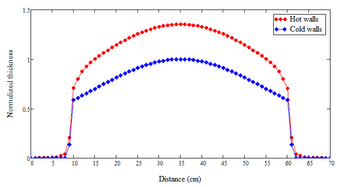
Figure 4
As shown in Fig. 4, there is a substantial gain, roughly 35%, in the deposition rate when the walls are hot, compared to cold walls. Another visible difference is in the manner of thickness roll-off near the borders defined by the front and back wall: with hot walls the roll-off is more gradual than that for cold walls.
To correct the thickness nonuniformity, we can introduce a pair of masks that protrude into the deposition zone from the two ends (shown in Fig. 2). These masks are optimized to correct a major portion of the 50-cm span when hot walls are present: the resultant thickness distribution is shown in Fig. 5. The same correction masks do not effectively flatten the thickness distribution if the walls are cold, also shown in the figure.
If a mask pair is optimized for cold walls it will, in this example, overcorrect the thickness distribution produced by the hat walls.
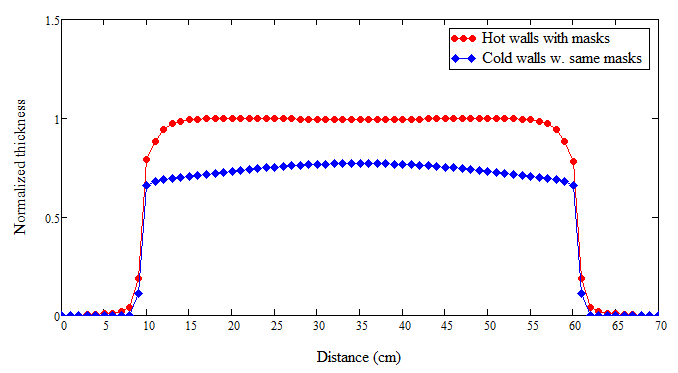
Figure 5
Another important difference between cold and hot walls is in the incident-angle statistics: substantially more vapor particles arrive at large angles when the walls are hot. Such difference can be consequential because incident-angle distributions affect the atomic stacking of a growing material. Furthermore, if area-defining shadow masks are employed, as in fabrication of OLED panels, the two types of partition walls can result in significantly different 3D profiles of the deposited materials: a discussion of the subject was posted on a Tin Model webpage.
(Statistics of the incident angle is a standard output of V-Grade 5S series software.)
In some manufacturing processes, whether partition walls are hot or cold may not be obvious. For example, some walls are not deliberately heated but heat transfer from the source (through conduction and/or radiation) make them partially condensation free. In such cases, the walls should be treated in more nuanced manners so that a numerical model maintains a high degree of realism.
We would like to hear your feedback on this subject. Please contact us at Tin Model LLC.